Hello, Welcome to MissouriView!
About
↓
About
This page will include tutorials that users can follow to bolster their understanding of remote sensing, GIS, and Machine Learning/Artifical Intelligence, all in a real-world and application-driven playground. Look for yourself, a few of our tutorials are listed below. Happy learning!
The mission of the Missouri chapter of AmericaView is to promote and advance the use of remote sensing technology and data across the state of Missouri. MissouriView is here to do just that! The geospatial ecosystem is booming in Saint Louis. One entity advancing geospatial aptitude is the Geospatial Institute at Saint Louis University. With a cross-cutting cirriculum, GeoSLU is at the forefront of geospatial innovation. Below you will encounter a few tutorials developed at the Geospatial Institute by GIS practicioners. The current available tutorials are 1) Forest Conservation with AI, 2) Water Disparity and Levee Management, and 3) Missouri as Art.
Partners
↓
Partners
Forest Conservation with AI
↓
Forest Conservation with AI
In this course module, students are first introduced traditional machine learning including random forest (RF), support vector machine (SVM), and pixel-based deep learning using forest cover mapping in Madagascar as a case study. Then, the Convolutional Neural Network (CNN) approach is introduced, which utilizes spectral, textural and spatial information from WorldView-3 VNIR and SWIR data for classification and forest cover mapping in a fully automated learning process. The CNN approach used in this lab is U-Net (similar to Object-Based Image Analysis, OBIA in the remote sensing field. By completion of this lab, students can understand pros and cons of pixel-based (SVM, RF, DNN) and CNN-based OBIA; students also investigate forest change and impacts of human geography and conservation efforts on preserving forest habitats in Madagascar. You can access the data for this tutorial on our github page.
Area of Interest
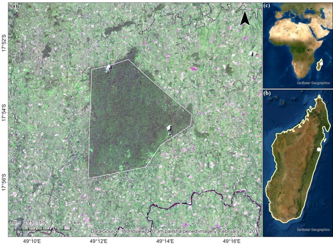
The study area is the Betampona Nature Reserve (BNR), outlined by the white boundary in Figure 1
(a).
The BNR is located in the eastern coast of Madagascar; the surrounding areas and the nature
reserve make
up of about 100 square km. This is a species rich area which provides the researchers with a
“living laboratory”
for the studies of human-forest interactions.
Madagascar houses a lively and diverse ecosystem, but due to encroachment,
deforestation tactics (illegal logging), aggressive agricultural practices and
urbanization, the environment has greatly altered. Additionally, with the presence
of invasive species such as Molucca Raspberry, Madagascar Cardamom, and Strawberry
Guava, biodiversity continues to be threatened.
Data Processing
| File Name | Description |
|---|---|
| Bet_LandCover_2019.tif | This is the “gold-standard" land cover/use map of the study area produced by object-based classification/segmentation of WV-3 imagery and significant post-processing and manual investigation using field surveys and ancillary data. |
| Bet_LandCover_2010.tif |
Classification map of the BNR and surrounding areas in 2010, created using
IKONOS-2 and Hyperion image analysis. Ghulam, A., Porton, I., Freeman, K. (2014). Detecting subcanopy invasive plant species in tropical rainforest by integrating optical and microwave (InSAR/PolInSAR) remote sensing data, and a decision tree algorithm. ISPRS Journal of Photogrammetry and Remote Sensing, 88: 174-192. |
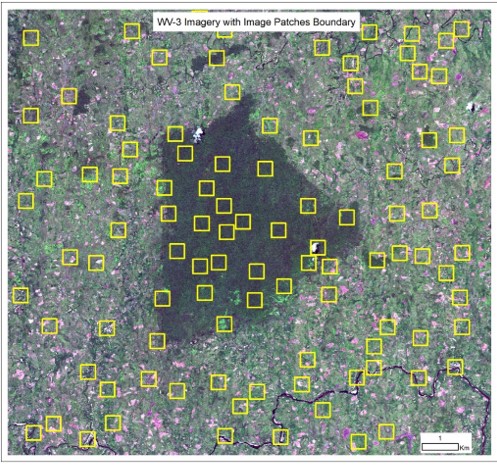
| Polygon.shp | This polygon represents the boundary of image patches, which will be later used to train the U-Net architecture and evaluate the results. There are a total 100 features in the polygon shapefile. |
| WV3_19Feb2019_BNR.tif |
16 band WorldView-3 imagery in reflectance including VNIR and SWIR bands, which are
atmospherically and radiometrically corrected and orthorectified. WV-3 VNIR and SWIR ground sampling distance (GSD) is 1.2 m and 3.7 m, respectively. VNIR-SWIR bands are layer-stacked and resampled to VNIR resolution using nearest-neighbor resampling. The SWIR bands can detect non-pigment biochemical phenomenon within plants including water, cellulose, and lignin. SWIR-4 (1729.5 nm), SWIR-5 (2163.7 nm), and SWIR-8 (2329.2 nm) can identify absorption phenomenon of nitrogen, cellulose, and lignin, respectively. The data were obtained from MAXAR through priority satellite tasking during the experiment. |
The original ground truth data were collected in the field using GPS surveys.
A total of nearly 400 polygons in different sizes and shapes and point samples
were collected. These ground surveys were used to produce the “gold-standard"
reference imagery (Bet_LandCover_2019.tif) as described in the published paper.
For this course module, however, we generated a new set of training samples
from the gold-standard reference imagery to simplify the implementation.
First, observe the following map:
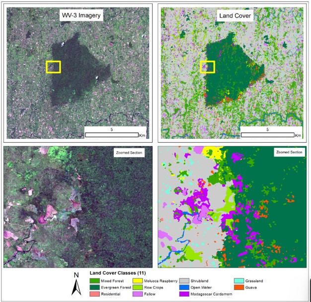
As stated above, the WV-3 image contains 16 bands. Further details about the 16 bands can be found in Cota et al. (2021). There are a total of 11 land cover classes that were created by CNN-based image segmentation. That means all pixels in the study area already classified as some land cover/use type. The codes for each land cover class are given below:
| Int Code | Class |
|---|---|
| 1 | Mixed Forest |
| 2 | Evergreen Forest |
| 3 | Residential |
| 4 | Molucca Raspberry |
| 5 | Row Crops |
| 6 | Fallow |
| 7 | Shrubland |
| 8 | Open Water |
| 9 | Madagascar Cardamon |
| 10 | Grassland |
| 11 | Guava |
U-NET requires image patches or image chips as input data. To create this data for
this tutorial, we generated a polygon shapefile, named ‘polygon.shp”, based on the
gold-standard land cover/use map. This polygon represents the boundary of image
patches, which will be later used to train the U-Net architecture and evaluate the
results. There are a total of 100 features in the polygon shapefile. The steps to
generate these training samples are below.
1. Create a set of randomly generated points using ArcGIS Pro. To do this,
open ArcToolbox and open the Data Management
Tools > Feature Class > Create random points tool.
2. Create a circular buffer around those points, set buffer size to 192 meters.
3. Convert the circle to a square-shaped polygon by using “Minimum Bounding Geometry”
tool and use “Envelope” as the geometry type
Steps
Please go through all the provided DEMO notebooks:
- UNET_part1A_preprocessing_DEMO.ipynb
- Demonstrate the preprocessing steps.
- After preprocessing, save the train and test set in npy format.
- UNET_part1B_training_DEMO.ipynb
- Perform the training of UNET.
- Save the best model.
- UNET_part1C_applying_model_to_map_DEMO.ipynb
- Apply the model to the whole image.
- Divide the image into similar size image patches.
- hen apply model to each patch.
Assignment
Write a report (no more than 4 pages) about the methods and results from this lab.
You can rely on the Cota et al. (2021) publication for reference, but note that the
goal for this report is how the U-Net worked and how you implemented it. Focus on how
each segment of code worked and what are the 5 key skills you learned about CNN and
U-NET. You can include figures but do not fill up the whole report with just figures.
Here is a template you can follow:
- Introduction: Talk about the background behind the task. Why are you doing this? What are you expecting from the model? The objectives.
- Methods: (Try to create a short figure showing the overall workflow)
- Preprocessing: How did you preprocess the data. Try to briefly describe the tasks of the codes provided in the notebook
- U-NET Training: How many parameters were there? What hyperparameter values you used? What loss function and optimizer you used and why?
- Applying to Image: How did you apply the model to the whole image?
- Results: What is the overall accuracy? Show the confusion matrix, kappa scores and other metrics you want to show.
- Discussion: is this a segmentation or classification approach? What are the advantages and disadvantages between the two? Did U-NET utilize spectral information? What about texture and spatial patterns?
- Conclusion: What did you achieve? What are the possible next steps that can improve
the results?
Use Time New Roman / Arial / Calibri with 11 pt font size. Use default line spacing (Multiple, 1.08). Letter page.
Grading Scale
| Task | Percentage |
|---|---|
| Run code correctly, generate all figures | 50% |
| Introduction
|
5% |
| Methods
|
20% |
| Results
|
10% |
| Discussion
|
10% |
| Conclusion | 5% |
Assessing Flood Impact with Levee Elevation Modeling
↓
Assessing Flood Impact with Levee Elevation Modeling
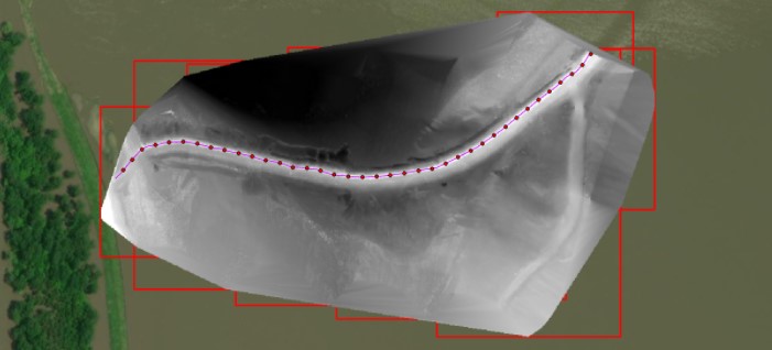
Typically, issues of water equity are associated with drinking water quality, but in cases of mismatched levee management plans water equity issues also arise when certain levees are managed and upgraded while others are not. In this example, the Len Small Levee in southern Illinois, a 17.2 mile-long levee managed by the local farmer’s bureau protecting $8.79 million of property, 13,500 acres that benefit 1400 local residents. The levee has repeatedly been breached since its construction in the 1940’s, and its reconfiguration in 1982. You can access the data for this tutorial on our github page. You can access the tutorial instructions in the google drive folder here and you can download the tutorial data here
.
What is a Levee?
A levee is a flood-control structure erected in order to prevent flood waters from inundating specific areas of land. The Len Small Levee, aside from protecting valuable farm land from flooding, is a deflection levee. Deflection levees control the paths of rivers. The Len Small Levee controls the current path of the Mississippi River by deflecting its path from crossing the narrow swath of land forming the narrow switchback, or meander bend, known as Dogtooth Bend. Insert pic here, if need be.
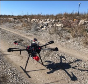
Technological Background: Drone Based LiDAR
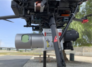
To get an accurate elevation, the LiDAR system has a built-in GPS system. During the Lidar survey, a GPS unit recorded the position and orientation of the sensor so that the Lidar point cloud can be used to calculate a Digital Elevation Model rather than only terrain.
Deliverables
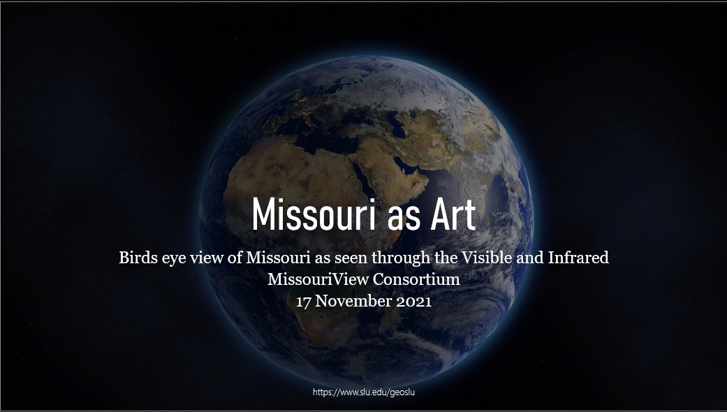
Missouri as Art
↓
Missouri as Art
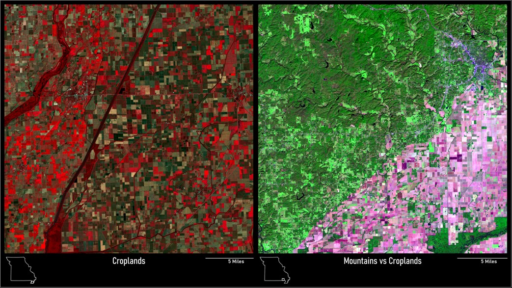
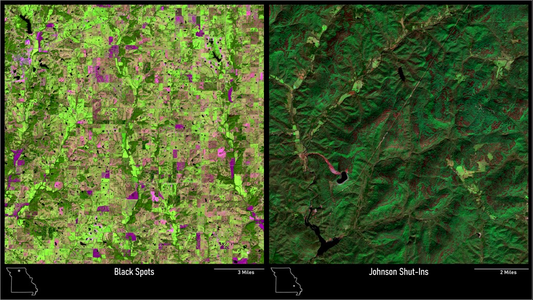
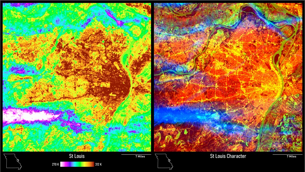
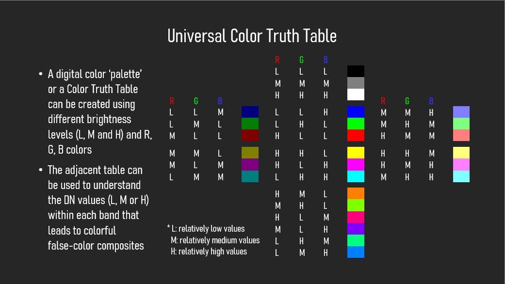
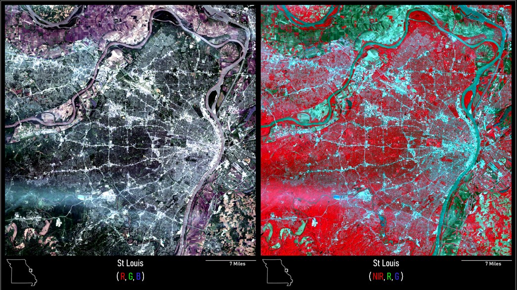
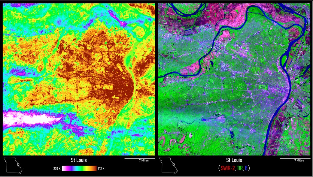
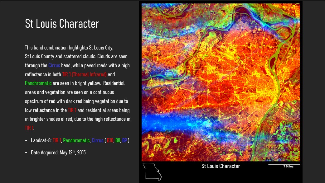
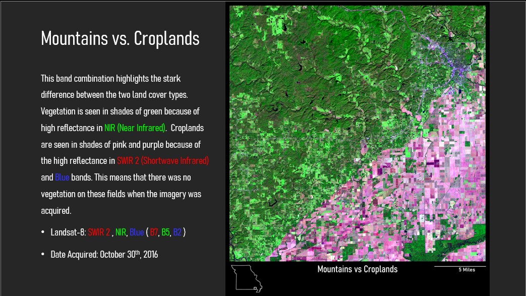
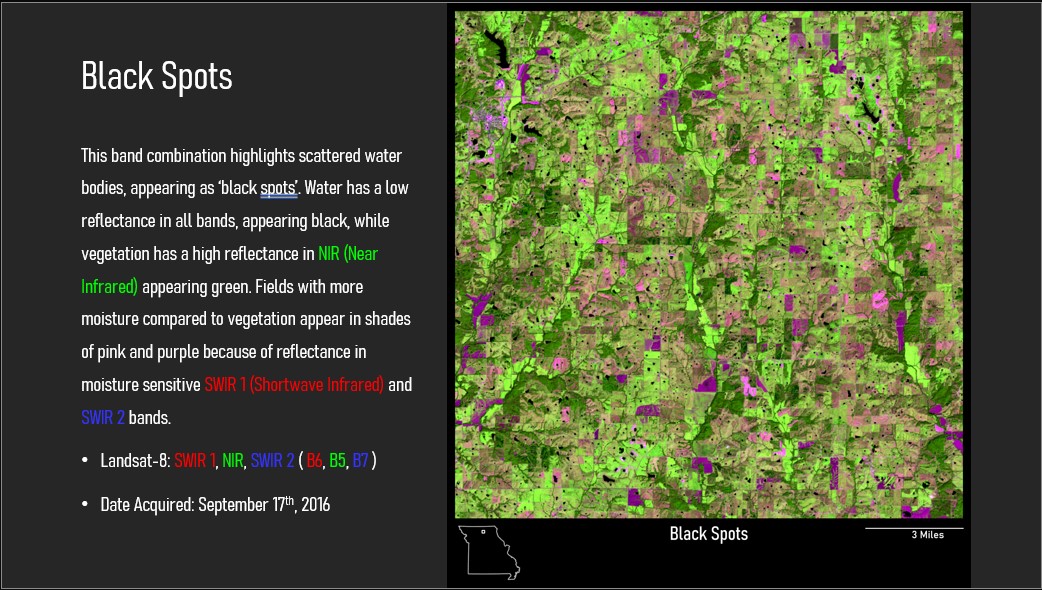
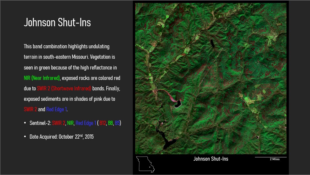
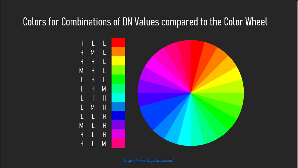
Missouri is a naturally beautiful state, and one of
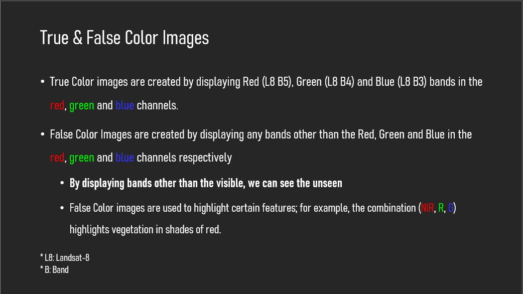
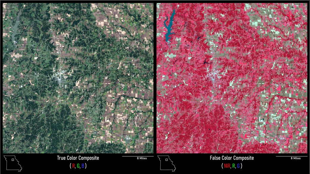
the most stunning ways to visualize Missouri’s beauty is by using different
multispectral band combinations to optimize the visualization of remote sensing data
to highlight different features on the ground. The Missouri as Art portion of MissouriView’s
mission makes remote sensing data more visually intriguing and artistic for building interest
from K-12 communities, while introducing students to applied concepts in remote sensing.
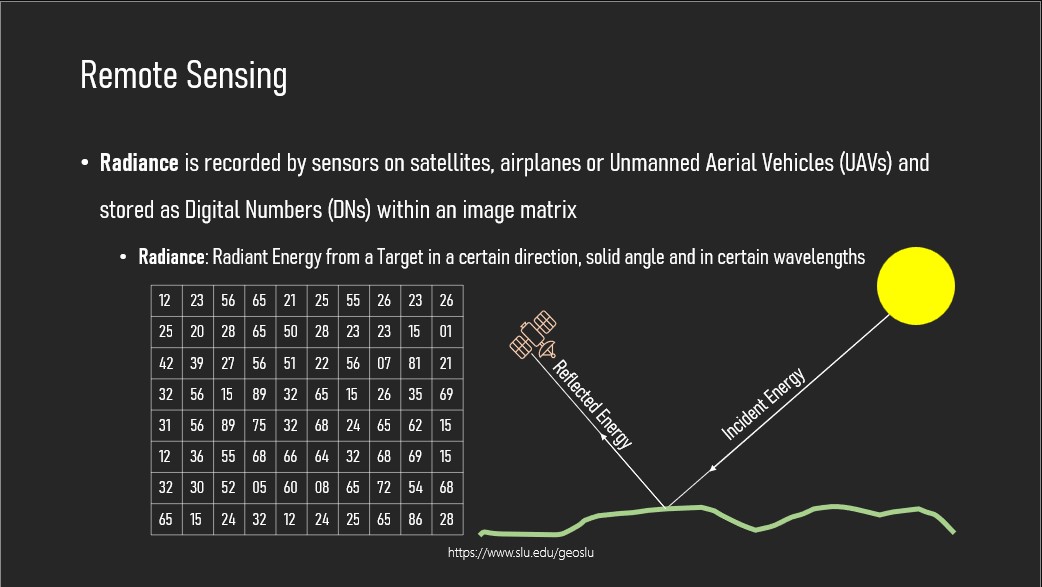
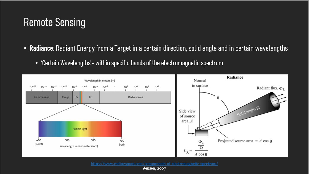
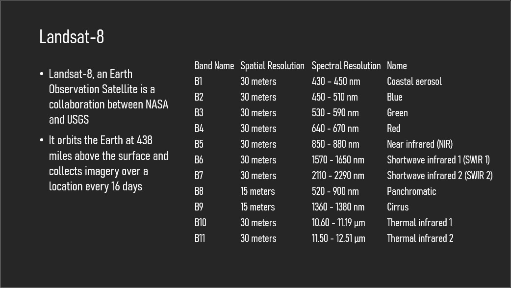
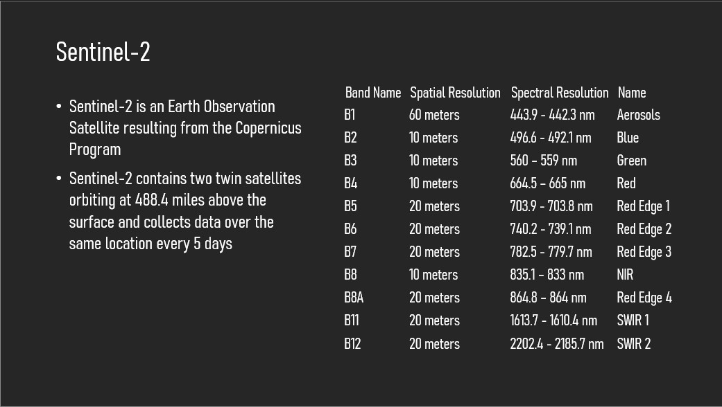
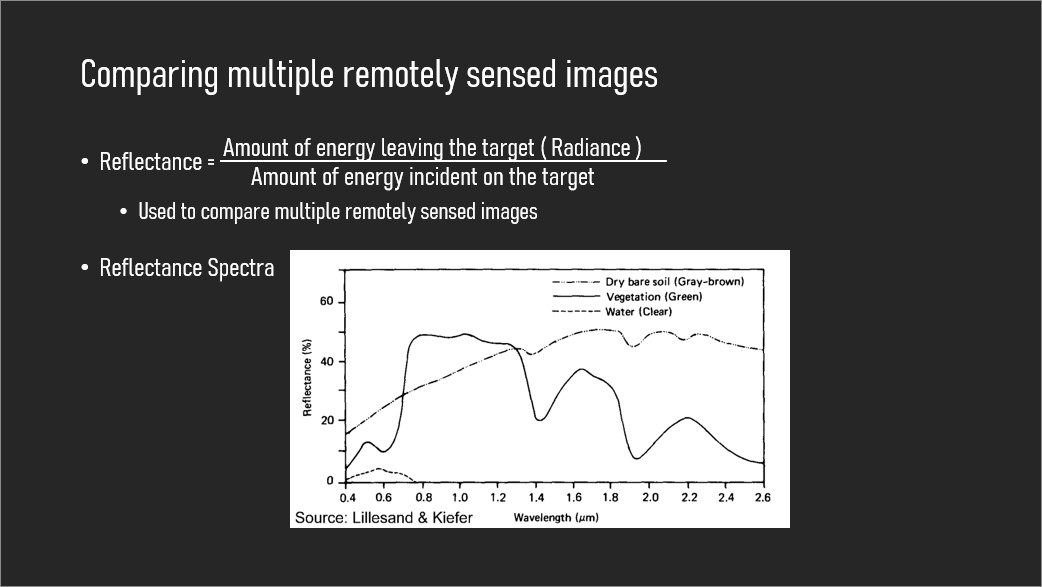
Here, students are introduced to the Electromagnetic Spectrum, the concepts of remote sensing
bands, how different bands are visualized, and how different combinations of bands can
highlight features of different types (i.e. water, agriculture, mineral exploration and
extraction, etc...).
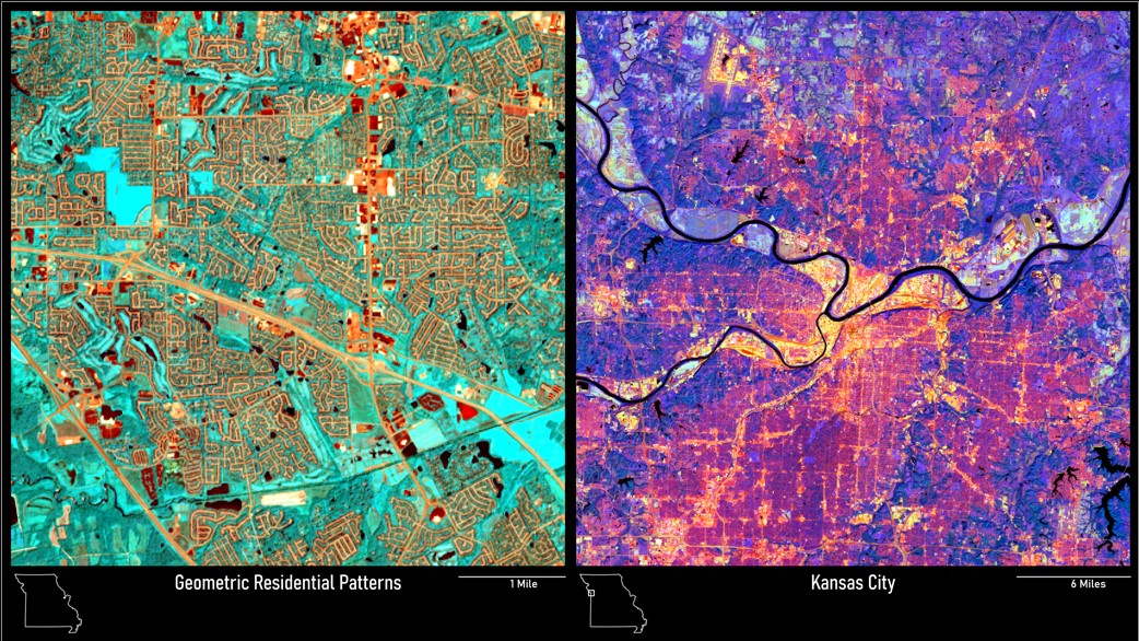
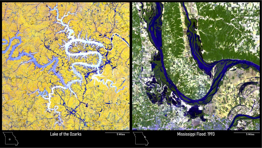
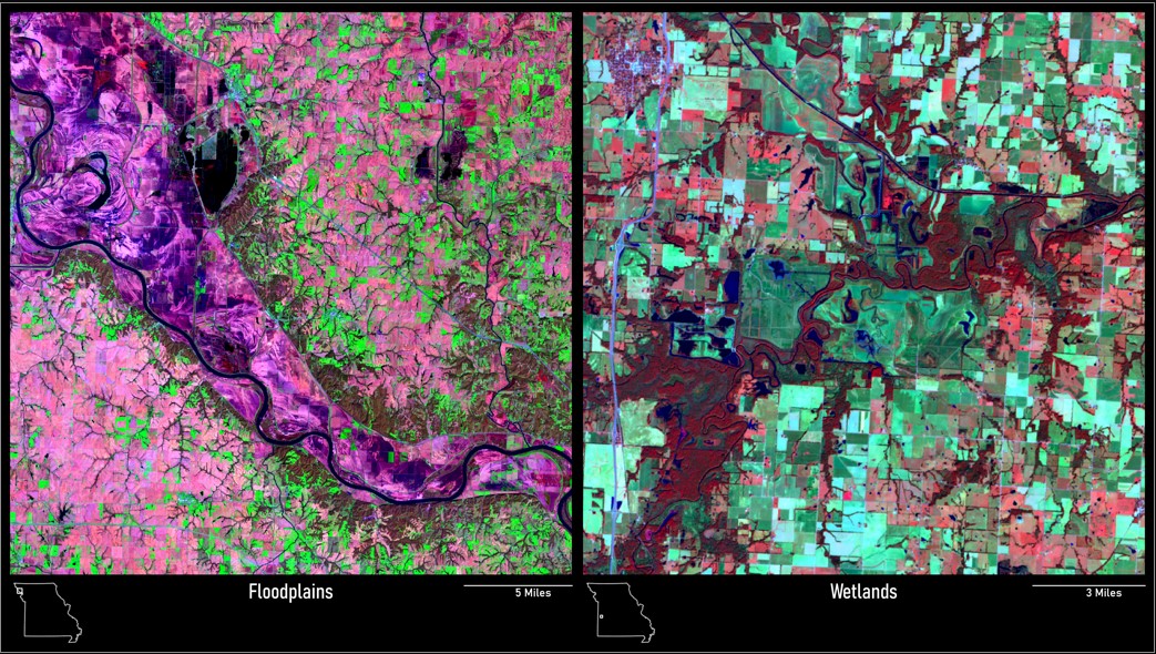
Power point material provides introduction to remote sensing with ample
examples of imagery collected in Missouri. With intuitive combination of satellite imagery,
the material highlight distinct Missouri landscape, ideal training material for K-16. You can
access our github
page to download the PPT.
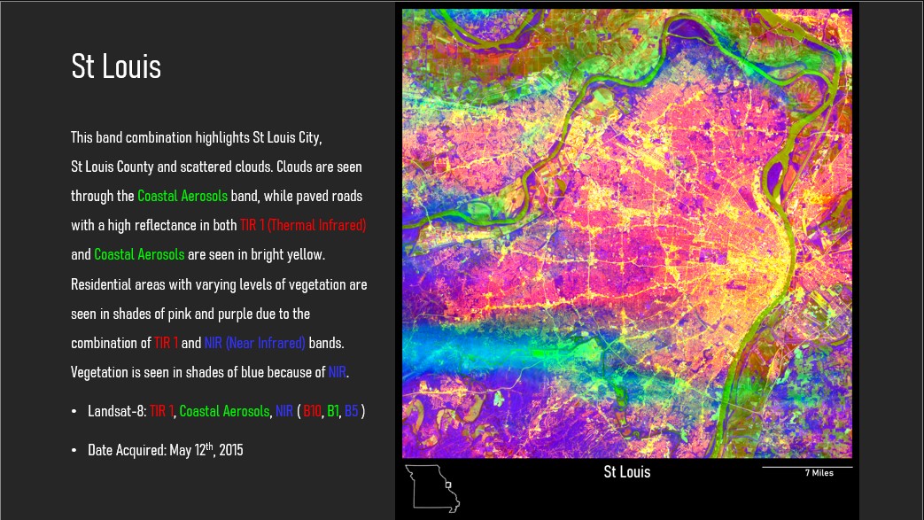
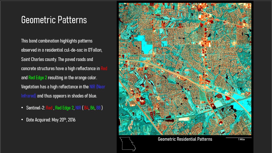
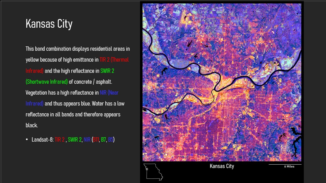
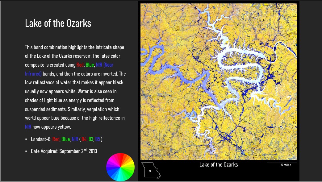
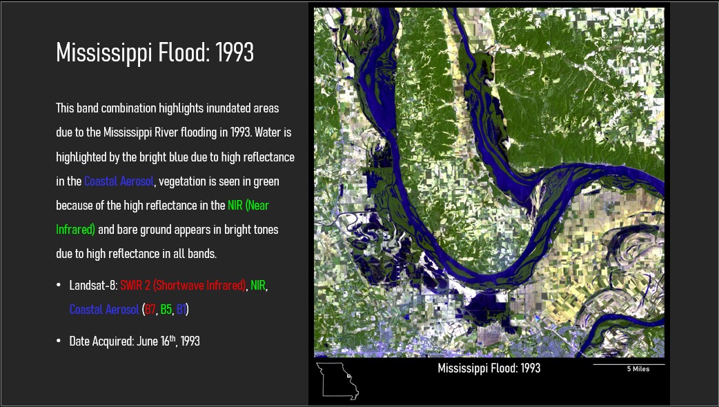
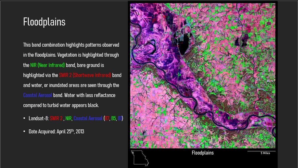
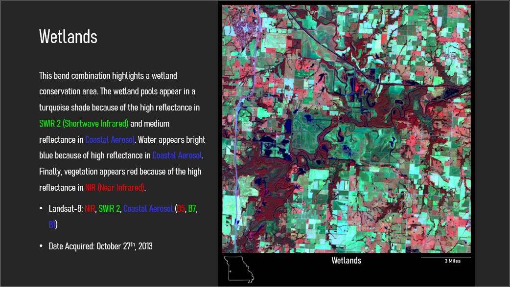
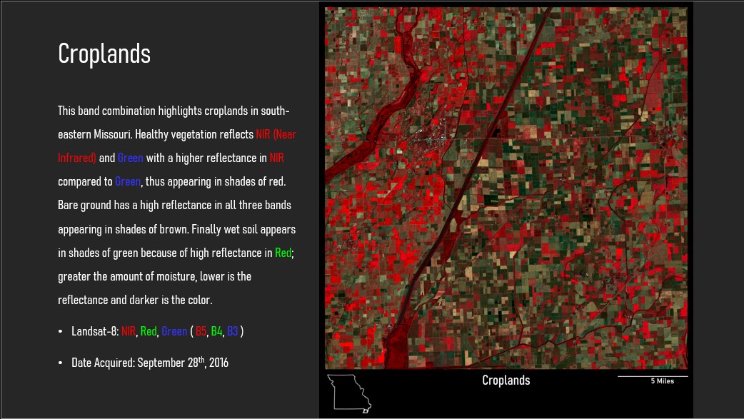
Slide Show